🦾 PINNs in Continuum Robotics

The use of PINNs has been explored for modeling deformations of continuum robots for sample-based path planning by Bensch et al. (2024), which previously was thought to be extremely computationally expensive. The team modeled a static Cosserat rod PINN for a tendon-driven continuum robot.

Continuum robots (CRs):

• used for inspection tasks in confined spaces, slow moving (which his why static is usually fine)
• the Cosserat rod theory is usually used to model tendon driven continuum robots (TDCRs)
  • demanding in compute
• path-planning algorithms for CR make therefore use of simple kinematic models, because often the model needs to be computed frequently
• disadvantages:
  • sim-to-real gap with purely kinematic models, specifically for the non-linear and non constant-curvature (CC) shapes
• PINNs can model the entire continuous shape given the actuation, instead of learning actuator to end-effector mappings
  • important for collision detection

As stated, the Cosserat Rod Theory is a maths framework that the modeling of slender and flexible structures commonly relies upon. It differs from its predecessors, such as the Euler-Bernoulli beam theory or Timoshenko beam theory, in that it accounts for 6 degrees of freedom. The maths behind these models is covered below.

Since Bensch et al. (2024), however, other developments in the space of continuum robotics and PINNs have been published. Krauss et al. (2024), for example, decoupled time from the network and used closed-form gradients instead of autodiff, enabling faster training on larger dynamical systems. Their architecture is know as DD-PINN.

Licher, Bartholdt, Krauss et al. (2025) applied the DD-PINN to dynamic Cosserat rod and used inside MPC at 70 Hz with an Unscented Kalman Filter (UKF) for state estimation. This was the first real-world dynamic control of a soft continuum robot using a Cosserat PINN.

The UKF is needed for state estimation in work by Licher, Bartholdt, Krauss et al. (2025).

• In the real world, one can't measure the full Cosserat rod state, i.e. its position, orientation, strains at every point along the rod. The tip position can only be located with a camera or sensor.
• The DD-PINN is used within an UKF for estimating the model states and bending compliance from end-effector position measurements. The UKF uses the DD-PINN as its internal model to propagate state predictions forward, then corrects them with the tip measurements.
• It also estimates the bending stiffness online, i.e. the model adapts if the real robot's stiffness differs from what was assumed during training.

---

The Euler-Bernoulli beam theory makes the assumption that the cross-sections of the structure remain plane and perpendicular to the centerline as it deforms. For slender beams where deflections are tiny, shear is negligible, and where a single constraint coupling bending and curvature is acceptable, the theory works well. The only real degrees of freedom per cross-section are position and bending rotation.

Let's examine a beam along the x-axis with transverse (perpendicular to the beam axis) displacement w(x,t):

The rotation of the cross-section is dependent on the deflection:

$$\theta(x,t) = \frac{\partial w}{\partial x}$$

The curvature or the bending strain is then defined as

$$\kappa = \frac{\partial^2 w}{\partial x^2}$$

The bending moment becomes

$$M = EI\kappa = EI\frac{\partial^2 w}{\partial x^2}$$

It states that the bending moment at any point is proportional to the local curvature, with the proportionality constant EI, also referred to as flexural rigidity.

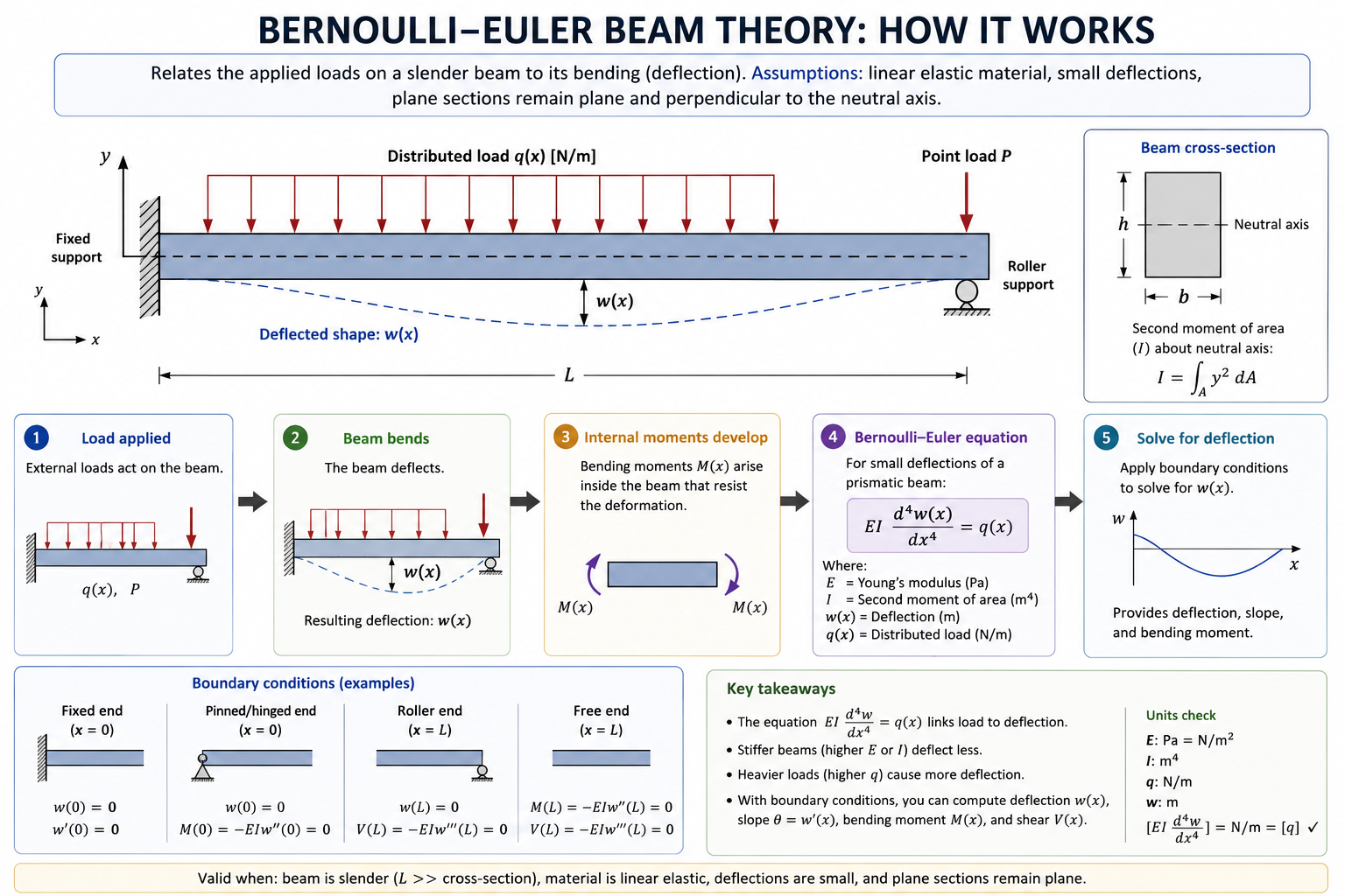
Therefore, the governing equation is therefore a classic 4th-order PDE:

$$EI\frac{\partial^4 w}{\partial x^4} + \rho A\frac{\partial^2 w}{\partial t^2} = q(x,t)$$

where E is Young's modulus (material stiffness), I is second moment of area, ρA is mass per unit length, q is distributed load. Note: this is the dynamic form of the PDE with an additional inertia term, which is just just Newton's second law (F = ma)

$$\rho A\frac{\partial^2 w}{\partial t^2}$$

In the static case, this term would be zero because there is no acceleration.

If a PINN were to be built using the (dynamic) Euler-Bernoulli model, it would take (x, t) as an input and output w(x, t).

The physics loss would be the the mean squared residual over a bunch of sampled collocation points:

$$\mathcal{L}_{\text{physics}} = \frac{1}{N}\sum_{i=1}^{N}\left(EI,\frac{\partial^4 \hat{w}}{\partial x^4}\bigg|_{(x_i,t_i)} + \rho A,\frac{\partial^2 \hat{w}}{\partial t^2}\bigg|_{(x_i,t_i)} - q(x_i, t_i)\right)^2$$

computed via both 4th-order spatial derivatives and 2nd-order time derivatives via autodiff.

Quantity	Expression	Physical meaning
w(x)	w	Deflection — how far the beam has moved
dw/dx	w'	Slope — the angle of the beam at that point
d²w/dx²	w''	Curvature — how sharply the beam is bending
EI·w''	M(x)	Bending moment — internal couple resisting bending
EI·w'''	V(x)	Shear force — internal transverse force
EI·w''''	q(x)	Applied distributed load

---

According to the Timoshenko beam theory, the cross-section is allowed to rotate irrespective of the centerline tangent. This leads to the introduction of another separate variable, i.e. transverse shear strain, leaving two independent fields instead of just one, as was in the case of the Euler-Bernoulli beam theory.

The main differentiator as stated before, is that now the cross-section rotation is independent of the centerline's slope. The difference can be represented with an angle:

$$\gamma = \frac{\partial w}{\partial x} - \psi$$

It measures how much the cross-section has tilted away from being perpendicular to the deformed centerline. In Euler-Bernoulli, γ = 0 by assumption.

The bending strain (i.e. curvature) therefore becomes

$$\kappa = \frac{\partial \psi}{\partial x}$$

The bending moment encompasses the bending strain, similar to Euler-Bernoulli's model

$$M(x) = EI\frac{d\psi}{dx}$$

Shear force is proportional to the shear angle, with the effective shear stiffness κₛGA:

$$V(x) = \kappa_s GA\left(\frac{dw}{dx} - \psi\right)$$

where G is the shear modulus, A is the cross-sectional area, and κₛ is the correction factor that accounts for the non-uniform shear stress distribution across the section. κₛ is needed, because in Timoshenko theory, the shear stress varies parabolically, but the theory assumes it is uniform across the cross-section, so a correction factor is needed to scale it down to match the true parabolic distribution.

The two governing (dynamic) PDEs are therefore defined as:

$$\kappa_s GA\left(\frac{\partial^2 w}{\partial x^2} - \frac{\partial\psi}{\partial x}\right) + q = \rho A\frac{\partial^2 w}{\partial t^2}$$ $$EI\frac{\partial^2 \psi}{\partial x^2} + \kappa_s GA\left(\frac{\partial w}{\partial x} - \psi\right) = \rho I\frac{\partial^2 \psi}{\partial t^2}$$

Translational inertia in the force equation and rotary inertia in the moment equation. Two coupled second-order PDEs in two unknowns: w(x,t) and ψ(x,t). So, for a PINN, the network would be fed (x, t) and output (ŵ, ψ̂).

Let's discuss the Timoshenko-based PINN in a little more depth. The network is a function:

$$\text{NN}: (x, t) \mapsto (\hat{w}, \hat{\psi})$$

Let's assume it's a single network with shared hidden layers rather than two separate networks.

From these two outputs we need to compute six derivative quantities (for a dynamic setup):

From ŵ:

• ∂ŵ/∂x (slope),
• ∂²ŵ/∂x² (for the force equation),
• and ∂²ŵ/∂t² (translational acceleration).

From ψ̂:

• ∂ψ̂/∂x (curvature),
• ∂²ψ̂/∂x² (for the moment equation),
• and ∂²ψ̂/∂t² (rotational acceleration).

Once these derivatives are computed, we can plug them into the two PDEs to find the residuals, which measure the degree to which the network violates the PDEs at each collocation point:

$$r_1(x,t) = \kappa_s GA\left(\frac{\partial^2 \hat{w}}{\partial x^2} - \frac{\partial \hat{\psi}}{\partial x}\right) + q(x,t) - \rho A \frac{\partial^2 \hat{w}}{\partial t^2}$$ $$r_2(x,t) = EI \frac{\partial^2 \hat{\psi}}{\partial x^2} + \kappa_s GA\left(\frac{\partial \hat{w}}{\partial x} - \hat{\psi}\right) - \rho I \frac{\partial^2 \hat{\psi}}{\partial t^2}$$

We also need boundary conditions at both ends of the beam, as well as the initial conditions (state and its time derivative):

$$\hat{w}(x,0) = w_0(x) \qquad \frac{\partial\hat{w}}{\partial t}(x,0) = \dot{w}_0(x)$$ $$\hat{\psi}(x,0) = \psi_0(x) \qquad \frac{\partial\hat{\psi}}{\partial t}(x,0) = \dot{\psi}_0(x)$$

In a dynamic setup, we sample points in the 2D domain [0, L] × [0, T]. The Bensch et al. (2024) paper used an adaptive strategy of resampling near the worst-performing regions after each epoch. PINNs are known to struggle with sharp features, but learn smooth regions easily, which is why this strategy was particularly effective.

The physics loss is therefore

$$\mathcal{L} = \lambda_{\text{phys}}\mathcal{L}_{\text{phys}} + \lambda_{\text{BC}}\mathcal{L}_{\text{BC}} + \lambda_{\text{IC}}\mathcal{L}_{\text{IC}}$$

where each component is:

$$\mathcal{L}_{\text{phys}} = \frac{1}{N}\sum_{i=1}^{N}\left[r_1(x_i,t_i)^2 + r_2(x_i,t_i)^2\right]$$ $$\mathcal{L}_{\text{BC}} = \frac{1}{N_B}\sum_{j=1}^{N_B}\left[\hat{w}(0,t_j)^2 + \hat{\psi}(0,t_j)^2 + \left(\frac{\partial\hat{\psi}}{\partial x}\bigg|_{L,t_j}\right)^2 + \left(\frac{\partial\hat{w}}{\partial x}\bigg|_{L,t_j} - \hat{\psi}(L,t_j)\right)^2\right]$$ $$\mathcal{L}_{\text{IC}} = \frac{1}{N_I}\sum_{k=1}^{N_I}\left[(\hat{w}(x_k,0) - w_0(x_k))^2 + (\hat{\psi}(x_k,0) - \psi_0(x_k))^2 + \left(\frac{\partial\hat{w}}{\partial t}\bigg|_{x_k,0} - \dot{w}_0(x_k)\right)^2 + \left(\frac{\partial\hat{\psi}}{\partial t}\bigg|_{x_k,0} - \dot{\psi}_0(x_k)\right)^2\right]$$

For our PINN, there might be several points of difficulty. Because the scaling factors for the force (κₛGA and ρA) and moment (EI and ρI) equations are drastically different by orders of magnitude, the two residuals will vary in magnitude, too - meaning that the smaller residual might get ignored by the optimizer, unless they are non-dimensionalised prior to forming the loss.

Bending and shear waves travel at different speeds. When the loss landscape is highly oscillatory, PINNs might struggle at learning the solutions. This is a known limitation.

The DD-PINN approach addresses another concern with PINNs that for long time horizons: it fails to capture at late times because the initial conditions doesn't propagate through the entire domain. This can be solved with windowing the time domain and training sequentially: solve [0, T₁] first, use the solution at T₁ as the initial condition for [T₁, T₂], and so on.

Causal training strategies, weighting earlier time points more heavily, or progressively expanding the time window during training, must also be taken into account when building the PINN.

---

The Cosserat rod theory models the rod as a 1D curve with a frame of directors attached at every point. At each point (per cross section), 6 degrees of freedom are tracked:

• 3 translational DOFs (position of the centerline),
• 3 rotational DOFs (orientation of the cross-section frame, typically parameterized via quaternions or rotation matrices).

Mathematically speaking, at every point s along the rod (with s being the arc length parameter, s ∈ [0, L]):

• the position of the centerline (3 DOFs) can be described as

$$\mathbf{r}(s,t) \in \mathbb{R}^3$$

• and the orientation of each cross-section (3 DOFs) as

$$\mathbf{R}(s,t) \in SO(3)$$

which is a 3×3 rotation matrix describing how the cross-section is oriented relative to the global frame (SO(3) is a set of all possible rotations in 3D space around a fixed point).

• SO(3) treats rotations using matrices (3x3 grids of numbers) or quaternions (4-element vectors) instead of simple angles.

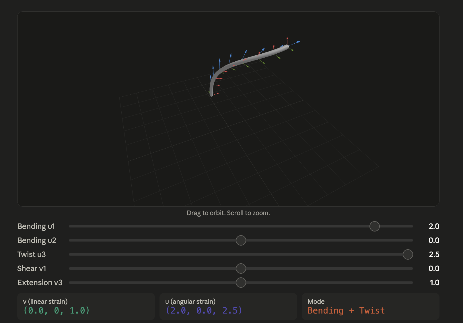
The spatial derivatives of r and R with respect to s describe the rod's deformation:

$$\frac{\partial \mathbf{r}}{\partial s} = \mathbf{R}\mathbf{v}$$ $$\frac{\partial \mathbf{R}}{\partial s} = \mathbf{R}[\mathbf{u}]_\times$$

So, the rate of change of position r along the rod is the rotation matrix applied to vector v.

• v is linear strain in the local frame.
  • v₁: shear strain in the local x-direction
  • v₂: shear strain in the local y-direction
  • v₃: axial stretch

The rate of change of orientation along the rod is R multiplied by a skew-symmetric matrix $[\mathbf{u}]_\times$ (the bracket notation $[\mathbf{u}]_\times$ just means its a skew-symmetric matrix).

• u is the angular strain (i.e. the curvature-twist vector) in the local frame.
  • u₁: bending curvature about the local x-axis
  • u₂: bending curvature about the local y-axis
  • u₃: twist per unit length about the local z-axis

The hat map $[\mathbf{u}]_\times$ takes a regular 3-vector u ∈ ℝ³ and turns it into a skew-symmetric matrix $[\mathbf{u}]_\times$ ∈ so(3).

Whilst SO(3) is the set of all 3D rotation matrices, so(3) is the Lie algebra of SO(3), i.e. the set of all 3x3 skew-symmetric matrices. So while SO(3) is the curved manifold of rotations, so(3) is the flat tangent space at the identity. It's a linear approximation of the curved surface near a point.

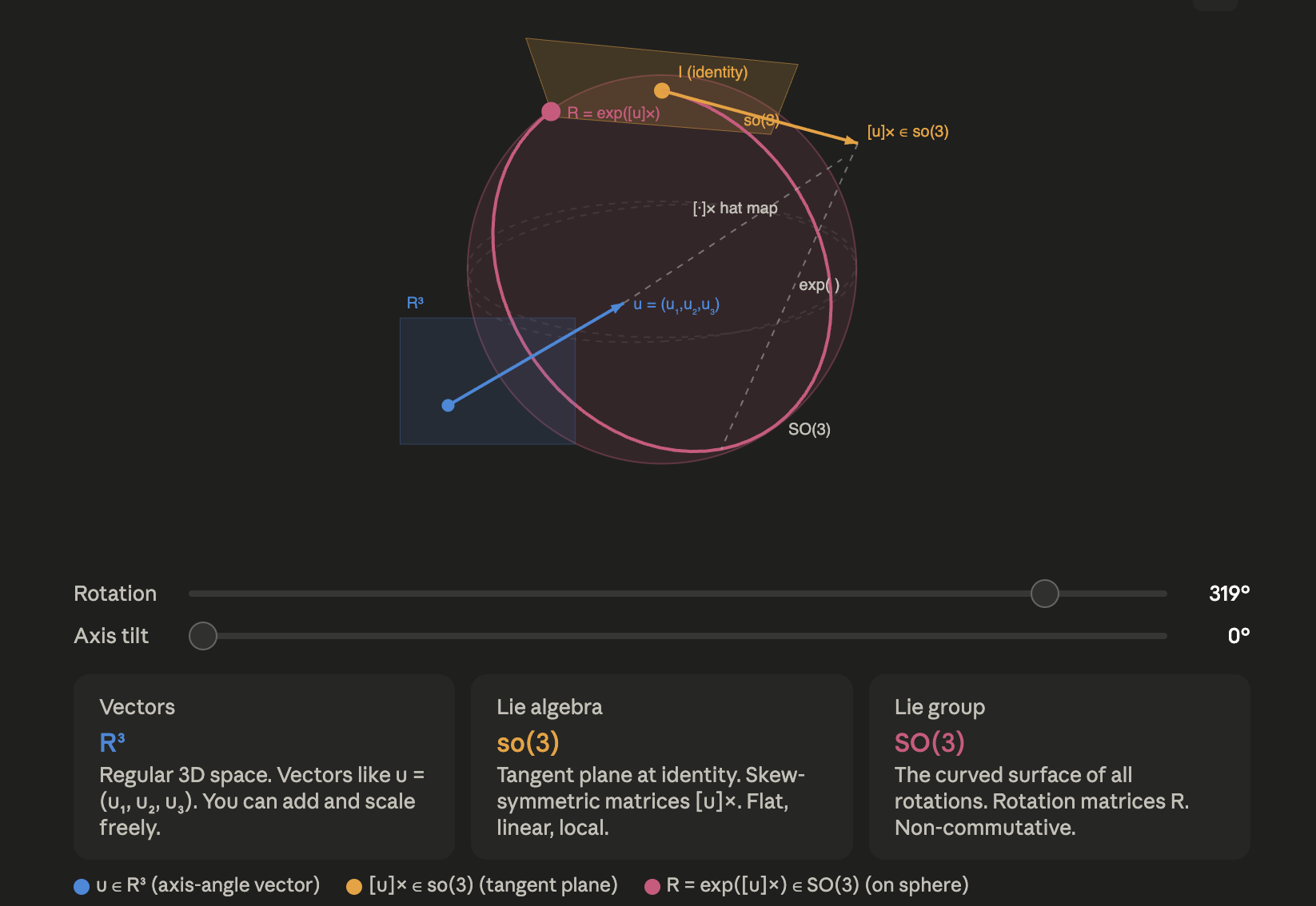
The skew-symmetric matrix $[\mathbf{u}]_\times$ lives in so(3), and it can be converted to an actual rotation in SO(3) via the matrix exponential: R = exp($[\mathbf{u}]_\times$). Going the other direction, i.e. from a rotation matrix back to the skew-symmetric matrix, is the matrix logarithm, which is what Bensch et al. used in their rotation distance metric:

$$d(\hat{R} R_{\text{Ref}}) = |\log(\hat{R}R_{\text{Ref}}^T)|$$

• They used the equation to measure how wrong the network's predicted orientation is compared to the reference orientation. It is difficult to penalize rotation errors when working in SO(3) rather than a vector space.
• The product of the network's predicted rotation R̂ and the transposed reference rotation $\mathbf{R_{\text{Ref}}^T}$ yields the relative rotation between the two, i.e. the single rotation that would take you from the reference orientation to the predicted orientation.
• The matrix logarithm was applied to the relative rotation to map it from SO(3) back down to so(3). The norm of that skew-symmetric matrix (or equivalently the norm of the 3-vector you extract from it) gives you the angle of the rotation needed to align the two frames.

Compare the Cosserat theory to two previous ones:

• In Euler-Bernoulli: v is locked to (0, 0, 1)ᵀ (no shear, no stretch), and u has only one nonzero bending component (2D bending). The single unknown w(x) determines everything.
• In Timoshenko: v can have nonzero v₁ or v₂ (shear allowed), but stretch is still locked (v₃ = 1), and again only planar bending. Two unknowns w and ψ.
• In Cosserat: all six components of v and u are free. Shear in two directions, extension, bending about two axes, and twist.

Both expressed in the global frame, the internal force n and moment m relate to the strains through the material law:

$$\mathbf{n} = \mathbf{R}\mathbf{K}_{se}(\mathbf{v} - \mathbf{v}_0)$$ $$\mathbf{m} = \mathbf{R}\mathbf{K}_{bt}(\mathbf{u} - \mathbf{u}_0)$$

where v₀ and u₀ are the undeformed reference strains, and the stiffness matrices are:

$$\mathbf{K}_{se} = \text{diag}(\kappa_s GA, \kappa_s GA, EA)$$ $$\mathbf{K}_{bt} = \text{diag}(EI_1, EI_2, GJ)$$

• $\mathbf{K}_{se}$​ handles shear and extension

  • κₛGA is the Timoshenko's shear correction factor
  • EA is the axial stiffness

• $\mathbf{K}_{bt}$​ handles bending and torsion

  • EI₁ and EI₂ are the bending stiffnesses about the two principal axes (they're equal for a circular cross-section)
  • GJ is the torsional stiffness

• The R out front rotates the body-frame constitutive response into the global frame.

The balance laws for a Cosserat rod are Newton's second law (F=ma) applied to each infinitesimal element, for both translation and rotation. These are the two governing PDEs for the dynamics Cosserat rod model.

For the linear momentum:

$$\frac{\partial \mathbf{n}}{\partial s} + \mathbf{f} = \rho A\frac{\partial^2 \mathbf{r}}{\partial t^2}$$

• The spatial derivative of internal force plus any external distributed force f equals mass per unit length times translational acceleration.

For the angular momentum:

$$\frac{\partial \mathbf{m}}{\partial s} + \frac{\partial \mathbf{r}}{\partial s} \times \mathbf{n} + \mathbf{l} = \rho\mathbf{J}\frac{\partial \boldsymbol{\omega}}{\partial t} + \boldsymbol{\omega} \times (\rho\mathbf{J}\boldsymbol{\omega})$$

• The spatial derivative of internal moment, plus the cross product of the position derivative with the internal force, plus external distributed moments l, equals the rate of change of angular momentum.

• The right side has two terms:

  • ρJ·∂ω/∂t is the angular acceleration term
  • ω × (ρJω) is the gyroscopic term that arises because the cross-section is spinning in 3D.

The angular velocity ω is extracted from:

$$[\boldsymbol{\omega}]_\times = \frac{\partial \mathbf{R}}{\partial t}\mathbf{R}^T$$

We've already seen something similar with the angular strain u, but this time its in terms of time t instead space s.

• So, instead of asking as I move along the rod (in s), how is the cross-section rotating, we are asking as time passes (in t), how is the cross-section rotating.

Following the Rucker and Webster formulation that Bensch et al. (2024) used, you can combine everything into a system:

$$\frac{\partial \mathbf{r}}{\partial s} = \mathbf{R} \mathbf{v}$$ $$\frac{\partial \mathbf{R}}{\partial s} = \mathbf{R} [\mathbf{u}]_\times$$ $$\begin{pmatrix} \frac{\partial \mathbf{v}}{\partial s} \\ \frac{\partial \mathbf{u}}{\partial s} \end{pmatrix} = \begin{pmatrix} \mathbf{K}_{se} + \mathbf{A} & \mathbf{G} \\ \mathbf{B} & \mathbf{K}_{bt} + \mathbf{H} \end{pmatrix}^{-1} \begin{pmatrix} \mathbf{d}_{dyn} \\ \mathbf{c}_{dyn} \end{pmatrix}$$

Bensch et al. (2024) used statics only. For slow motion, the accelerations are negligible. The structure is identical to statics. What changes is the content of the forcing vectors. They come from the equilibrium equations above (linear and angular momentum). The c and d vectors are just those two equilibrium equations expanded, rearranged into the body frame and solved for the strain derivatives.

For a dynamics system, they'd look like this:

$$\mathbf{d}_{dyn} = \underbrace{\mathbf{K}_{se}\dot{\mathbf{v}}^* - [\mathbf{u}]_\times\mathbf{K}_{se}(\mathbf{v} - \mathbf{v}^*) - \mathbf{R}^T\mathbf{f}_e - \mathbf{a}}_{\mathbf{d}_{static}} + \rho A\mathbf{R}^T\frac{\partial^2 \mathbf{r}}{\partial t^2}$$ $$\mathbf{c}_{dyn} = \underbrace{\mathbf{K}_{bt}\dot{\mathbf{u}}^{*} - [\mathbf{u}]_\times\mathbf{K}_{bt}(\mathbf{u} - \mathbf{u}^{*}) - [\mathbf{v}]_\times\mathbf{K}_{se}(\mathbf{v} - \mathbf{v}^{*}) - \mathbf{R}^{T}\mathbf{l}_e - \mathbf{b}}_{\mathbf{c}_{static}} + \rho\,\mathbf{R}^{T}\left(\mathbf{J}\,\frac{\partial \boldsymbol{\omega}}{\partial t} + \boldsymbol{\omega} \times \mathbf{J}\,\boldsymbol{\omega}\right)$$

So, now let's think about making a PINN using a Cosserat rod model.

• R is a 3×3 matrix in SO(3) that can be represented in a PINN either via:
  • Quaternions: q ∈ ℝ⁴ with ‖q‖ = 1. Output 4 numbers, normalize. No singularities.
    • Angular strain extraction uses q directly:

$$\mathbf{u} = 2\mathbf{E}(q)^T\frac{\partial q}{\partial s}$$

- Axis-angle: θ ∈ ℝ³. Output 3 numbers, convert to R via Rodrigues formula. Singularity at ‖θ‖ = 0 and 2π. This is what Bensch et al. (2024) did, for example.
- Rotation matrix directly: via special architectures that enforce orthogonality. 

For dynamics, the model will input (s, t, τ), where s is arc length and τ is the actuation parameter(s) and t is time. The model will output $\mathbf{r̂}$(s,t) ∈ ℝ³, $\mathbf{q̂}$(s,t) ∈ ℝ⁴.

However, if using an architecture similar to a DD-PINN introduced by Krauss et al. (2024), which decouples the time domain from the neural network, time is not an input into the PINN. Instead, the model learns a single-step state transition: given the current state and input, predict the state a short time step later. This leads to much faster computation times, as it allows for closed-form gradient computation rather than autodiff through the time domain.

The derivatives for autodiff:

• From r̂:

  • ∂$\mathbf{r̂}$/∂s (for linear strain),
  • ∂²$\mathbf{r̂}$/∂s² (for strain derivative) and
  • ∂²$\mathbf{r̂}$/∂t² (translational acceleration).

• From q̂:

  • ∂$\mathbf{q̂}$/∂s (for angular strain),
  • ∂²$\mathbf{q̂}$/∂s² (for angular strain derivative),
  • ∂$\mathbf{q̂}$/∂t (for angular velocity) and
  • ∂²$\mathbf{q̂}$/∂t² (for angular acceleration).

The residuals for dynamics become

$$\mathbf{r}_1(s,t) = \frac{\partial \hat{\mathbf{n}}}{\partial s} + \mathbf{f} - \rho A\frac{\partial^2 \hat{\mathbf{r}}}{\partial t^2}$$ $$\mathbf{r}_2(s,t) = \frac{\partial \hat{\mathbf{m}}}{\partial s} + \frac{\partial \hat{\mathbf{r}}}{\partial s} \times \hat{\mathbf{n}} + \mathbf{l} - \rho\mathbf{J}\dot{\hat{\boldsymbol{\omega}}} - \hat{\boldsymbol{\omega}} \times (\rho\mathbf{J}\hat{\boldsymbol{\omega}})$$

The kinematic consistency residuals are the same as for the static case:

$$\mathbf{r}_3(s) = \frac{\partial \hat{\mathbf{r}}}{\partial s} - \hat{\mathbf{R}}\hat{\mathbf{v}}$$ $$\mathbf{r}_4(s) = \frac{\partial \hat{\mathbf{R}}}{\partial s} - \hat{\mathbf{R}}[\hat{\mathbf{u}}]_\times$$

• These enforce that the position and rotation derivatives are actually consistent with the strains the network is predicting. If you derive v and u purely from autodiff on $\mathbf{r̂}$ and $\mathbf{q̂}$, then r₃ and r₄ are automatically zero by construction.
  • But if the network outputs û as a separate head like Bensch et al. (2024) did, these consistency residuals are nonzero and must be enforced.

Boundary conditions (at s = 0 and s = L, for all t):

$$\hat{\mathbf{r}}(0,t) = \mathbf{r}_0 \qquad \hat{\mathbf{R}}(0,t) = \mathbf{R}_0$$ $$\hat{\mathbf{n}}(L,t) = \mathbf{n}_{applied}(t) \qquad \hat{\mathbf{m}}(L,t) = \mathbf{m}_{applied}(t)$$

Initial conditions (at t = 0, for all s):

$$\hat{\mathbf{r}}(s,0) = \mathbf{r}_0(s) \qquad \hat{\mathbf{R}}(s,0) = \mathbf{R}_0(s)$$ $$\frac{\partial\hat{\mathbf{r}}}{\partial t}(s,0) = \dot{\mathbf{r}}_0(s) \qquad \hat{\boldsymbol{\omega}}(s,0) = \boldsymbol{\omega}_0(s)$$

And finally the total physics loss:

$$\mathcal{L} = \lambda_1 |\mathbf{r}_1|^2 + \lambda_2 |\mathbf{r}_2|^2 + \lambda_3 |\mathbf{r}_3|^2 + \lambda_4 |\mathbf{r}_4|^2 + \lambda_{BC}\mathcal{L}_{BC} + \lambda_{IC}\mathcal{L}_{IC} + \lambda_q\mathcal{L}_q + \lambda_{data}\mathcal{L}_{data}$$

• The data loss $\mathbf{ℒ_{data}}$ is optional (was included by Bensch et al. (2024)).

References & Useful Reading

Bensch, M., Job, T.-D., Habich, T.-L., Seel, T., & Schappler, M. (2024). Physics-Informed Neural Networks for Continuum Robots: Towards Fast Approximation of Static Cosserat Rod Theory. In 2024 IEEE International Conference on Robotics and Automation (ICRA) (pp. 17293–17299). https://doi.org/10.1109/ICRA57147.2024.10610742

Krauss, H., Habich, T.-L., Bartholdt, M., Seel, T., & Schappler, M. (2024). Domain-Decoupled Physics-informed Neural Networks with Closed-Form Gradients for Fast Model Learning of Dynamical Systems. In Proceedings of the 21st International Conference on Informatics in Control, Automation and Robotics (ICINCO) (pp. 55–66). https://doi.org/10.5220/0012935200003822

Licher, J., Bartholdt, M., Krauss, H., Habich, T.-L., Seel, T., & Schappler, M. (2025). Adaptive Model-Predictive Control of a Soft Continuum Robot Using a Physics-Informed Neural Network Based on Cosserat Rod Theory. arXiv preprint, arXiv:2508.12681.

Jiahao, T. Z., Adolf, R., Sung, C., & Hsieh, M. A. (2024). Knowledge-based Neural Ordinary Differential Equations for Cosserat Rod-based Soft Robots. arXiv preprint, arXiv:2408.07776.

Schommartz, N., Klein, D., Alzate Cobo, J. A., & Weeger, O. (2024). Physics-augmented neural networks for constitutive modeling of hyperelastic geometrically exact beams. Computer Methods in Applied Mechanics and Engineering, 435, 117592. https://doi.org/10.1016/j.cma.2024.117592

Liu, J., Borja, P., & Della Santina, C. (2023). Physics-Informed Neural Networks to Model and Control Robots: A Theoretical and Experimental Investigation. Advanced Intelligent Systems.

Xun, L., Rosa, B., Szewczyk, J., & Tamadazte, B. (2025). A General Lie-Group Framework for Continuum Soft Robot Modeling. arXiv preprint, arXiv:2603.08232.